|
Sequia basalto
Understanding the drought phenomena in Uruguay and
developing a participatory methodology to improve the
resilience of livestock farmers of the Basalt region
Participants:
Danilo Bartaburu -
Instituto Plan Agropecuario, Salto, Uruguay. dbartaburu@planagropecurio.org.uy
Francisco Dieguez -
Instituto Plan Agropecuario, Montevideo, Uruguay. fdieguez@planagropecuario.org.uy
Jorge
Corral - Facultad de IngenierÃa, Montevideo,
Uruguay. jcorral@adinet.com.uy
Hermes
Morales - Instituto Plan Agropecuario, Salto, Uruguay.
paisanohermes@hotmail.com
Emilio
Duarte - Instituto Plan Agropecuario, Salto, Uruguay.
eduarte@planagropecuario.org.uy
Esteban
Montes - Instituto Plan Agropecuario, Salto, Uruguay.
emontes@planagropecuario.org.uy
Marcelo
Pereira - Instituto Plan Agropecuario, Salto, Uruguay.
pmsacra@adinet.com.uy
Pedro De
Hegedus - Faculdad de AgronomÃa, Udelar, Montevideo,
Uruguay. phegedus@adinet.com.uy
Pierre
Bommel - CIRAD and PUC University of Rio de Janeiro,
France and Brasil. bommel@cirad.fr
The Sequia
project is funded by INIA,
since May 2009.

Drought is one of the major events that causes negative
effects on livestock breeders in the basalt region. Most
livestock farms in the region are settled on basaltic
shallow soils. These soils have very limited capacity to
store water in their profile and are more sensitive to
drought. The severity and frequency of the droughts has
jeopardized the sustainability of ranches. In the late
1990s, livestock breeders experienced severe droughts
and millions of animals died or had to be slaughtered
prematurely. This led to a weakened beef production
sector causing numerous bankruptcies. Additionally, the
drought events may occur more frequently in the future
as a result of climate change.
To evaluate the efficiency of different management
strategies, we built an ABM to simulate the evolution of
farmers using different drought strategies. The purpose
of the ABM was to build prospective scenarios under the
assumption that future conditions (climate, prices) will
be similar to previous ones during the 2000-2009 decade.
Model purpose
The simulation model is designed to explore the impact
of different strategies on the trajectory of livestock
farms, especially taking into account the impact of
droughts. The first model is a standard ABM for which no
interactive simulation was planned. In that version,
agents are strong simplifications of farmers’ behaviors.
Two kinds of producers were considered depending on
their corresponding drought strategies:
- a “CC” Producer who
focuses on cattle health or on the Corporal Condition
score and
- a “Pasto” Producer who
makes drought-related decisions by assessing grass
availability and climate.
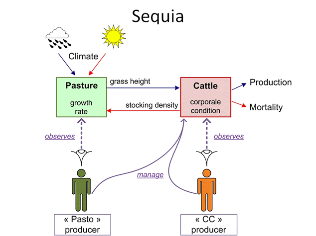
Whatever his strategy, a producer owns a 500 ha farm
composed of one single pasture (of a non-defined spatial
dimension). The grass grows according to the logistic
equation which parameters change according to seasonal
and climatic conditions. Two herds are grassing on the
farm: sheep that are not affected by drought (they are
able to survive even in extreme conditions) and for
which the dynamics is very simple, and cattle, which are
impacted by grass height and which lifecycle is more
finely modeled. The model consists of three submodels:
- The "Grazing "sub-model represents the grass growth
depending on the season and weather.
- The "wild" sub-model adds the herd that feeds on grass
and grows.
- The "management" sub-model adds a rancher who manages
his herd.
Model description
Model structure
The following class diagram presents the main classes
of the model:
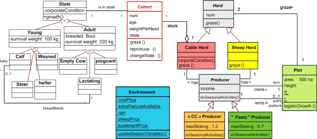
Whatever his strategy ("CC" or "Pasto"), a producer
owns a 500 ha farm composed of one single pasture (of a
non-defined spatial dimension). The grass grows
according to the logistic equation which parameters
change according to seasonal and climatic conditions.
Two herds are grassing on the farm: sheep that are not
affected by drought (they are able to survive even in
extreme conditions) and for which the dynamics is very
simple, and cattle, which are impacted by grass height
and which lifecycle is more finely modeled: the cattle
herd is made of cohorts of cows (a group of individuals
born at the same time period). When getting older, all
the animals of a cohort will growth and change their
state at the same time (calves, young adults then
reproductive adults). As they share the same
characteristics, we assume that they are similarly
affected by external events such as droughts. In other
words, the cohort agent is a cow plus a specific
attribute: number of animals of this cohort. The sheep
herd class is modeled as a simple entity without cohort,
but it has got an attribute (num, inherited by Herd
class) and even if its dynamics is very simple, it
grazes. Thus it has an effect on the grass height: each
sheep eats 2% of its weight per day. So the sheep herd
is a competitor to the cattle for grazing.
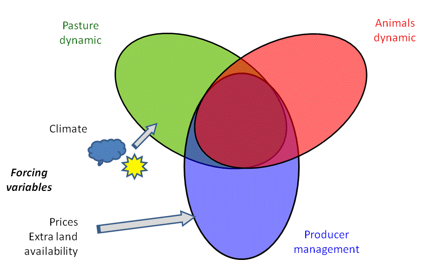
The model is deterministic but some input
parameters (climate data, meat prices, availability and
prices of extra farmland leasing of Environment class)
have been added as “forcing variables”. These time
series gathered during the 2000-2009 decade influence
the simulations: they play the role of one climatic and
market scenario for which various farmers’ management
strategies will be examined.
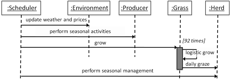
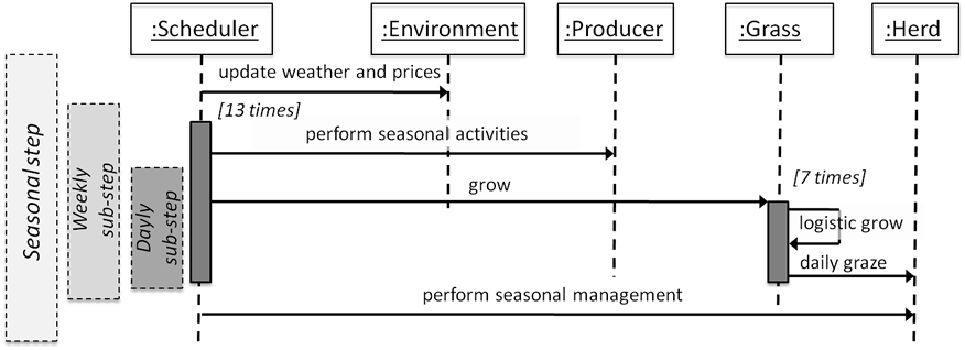
Time step
As the farmers have distinct seasonal activities, the
time-step for the simulations corresponds to one season.
But a one-day sub-step is needed to more accurately
represent the interactions between grass growth and
herds grazing (cattle and sheep). The task scheduling
order (i.e. order in which the behaviors of agents and
resources are called upon at every time step) is shown
on following sequence diagram:
By testing alternative strategies with the executable
editor, the participants identified some model biases:
they realized that in drought conditions, the agents
always reacted too late. For instance, in case of poor
health of the herd or in case of lack of grass, the
decision to feed the herd with supplement did not
apparently prevent it from collapsing. The participants
understood that during crises, the agents had to act
more frequently than only once per season as stated by
the first model version. The consequence being that we
intend to correct the model by repeating the seasonal
activities of the agents every week rather than only
once a season:
The states of a cohort
The following state-transition shows the life cycle of
a cohort of wild cattle with sub-states.
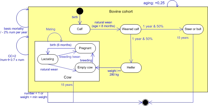
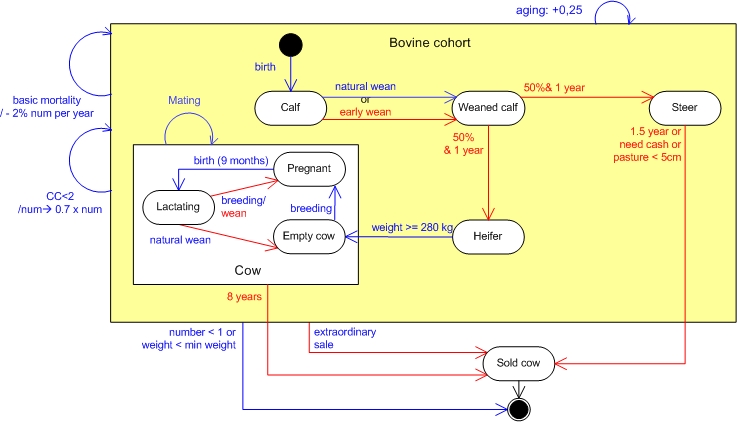
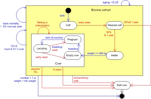
From this wild cattle model, 2 state-transition
diagrams are derived, showing the management events of
the producers. These human events are shown as red
transitions.
State-transition diagram of the "CC" producer, adapted
from previous diagram:
State-transition diagram of the "Pasto" producer:
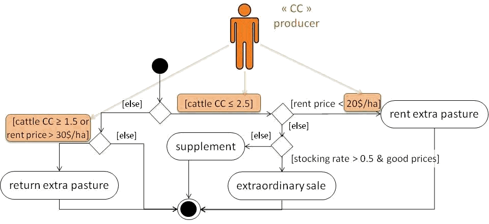
Producer activities
In the first version of the model, the activities have
been described as UML activity diagram: one diagram per
season and per agents strategy. The following diagram
presents the spring activities of a “Pasto” Producer
(green) and a “CC” Producer (orange).
These activities consist mainly in managing the farm
and the herds. Even if, for a given season, the
strategies are roughly similar, differences exist on the
decision points for each one: while the “CC” producer
surveys the physical condition of his cattle to guide
his managing choices, the “Pasto” producer chooses his
activities according to the grass height and by trying
to stay under a low stock threshold. The following
animated figure describes the behavior of both producers
(“Pasto” Producer: green and a “CC” Producer: orange)
during the spring season: even if they behave in the
same way, the guards (squared brackets) of the main
decision points concern the priority of each agent.
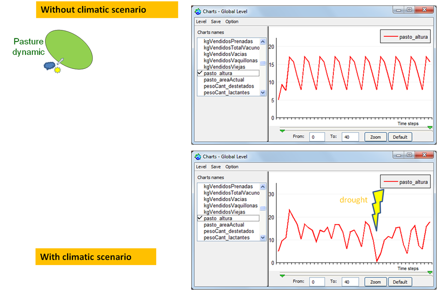
Some results
The following simulation curves show the evolution of
the pasture without grazing cattle, according to seasons
and climate:
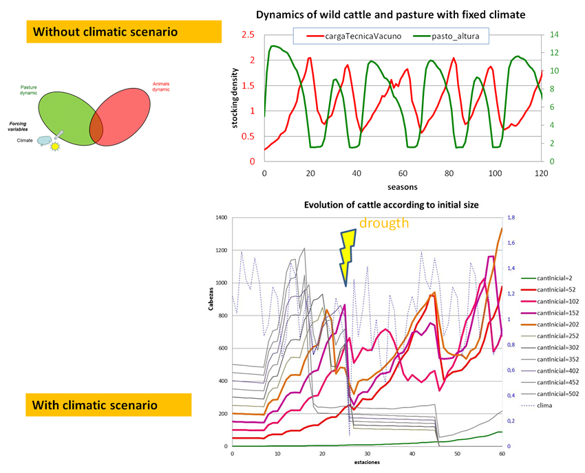
Result Pasture and wild cattle:
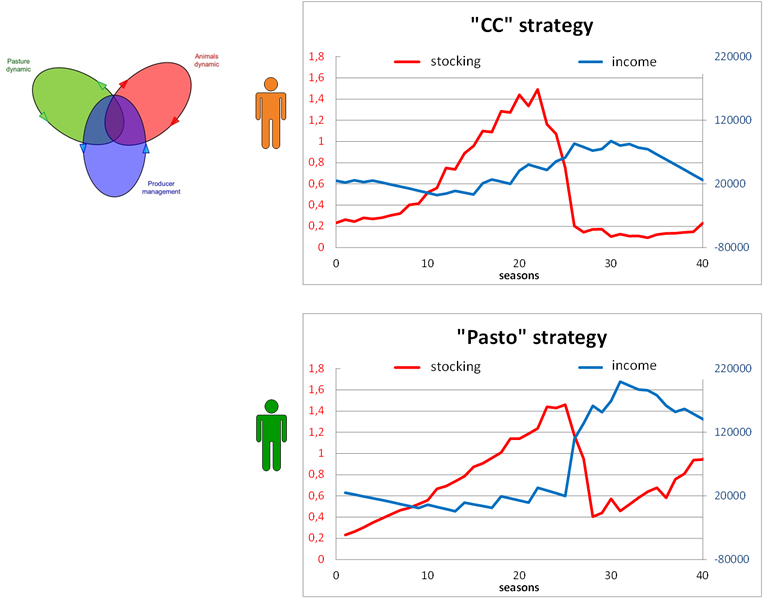
Some
result with producer management:
A more detailed description of the model will be
available soon.
The interactive model
To facilitate the collective design of the model, it
was necessary to immediately assess the consequences of
changes. For that purpose, we created a new tool that
enables the drawing of simple activity diagrams and to
execute them without any need for translation into code.
Indeed, this editor allows the creation of new activity
diagrams (or re-opening formers) that are interpreted
“on the fly” by Cormas. Then it is possible to modify
the simulator while it is running, without stopping or
restarting the simulation.
For simplicity sake and user friendliness, the elements
available on the diagram editor are restricted to
initial and final nodes, decision points, simple
activity nodes (without parameters nor ability to handle
an activity output) and transitions (Fig. 6). The
decision point has also limitations in the sense that
only two transitions come out of it, indicating the
fulfillment (true) or the negative answer (false) of a
test. The followinf figure presents the executable
Activity diagram editor displaying the spring strategy
for a collectively designed Producer. Note that this
diagram is equivalent to the one presented in the previous figure.
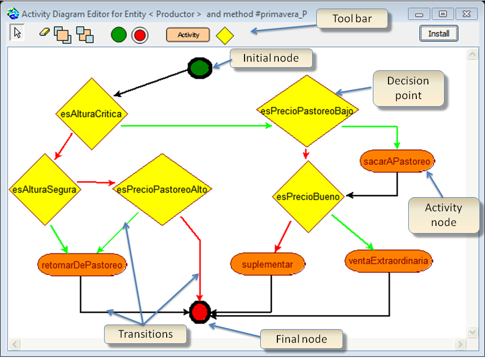
By selecting an activity node or a decision point on
the tool bar, the user can add a new element on the
diagram. Thereafter, he can choose the operation to be
performed by this element. Each element proposes a
drop-down menu to display an activity setter from which
the user may choose the method that will be associated
with the selected node
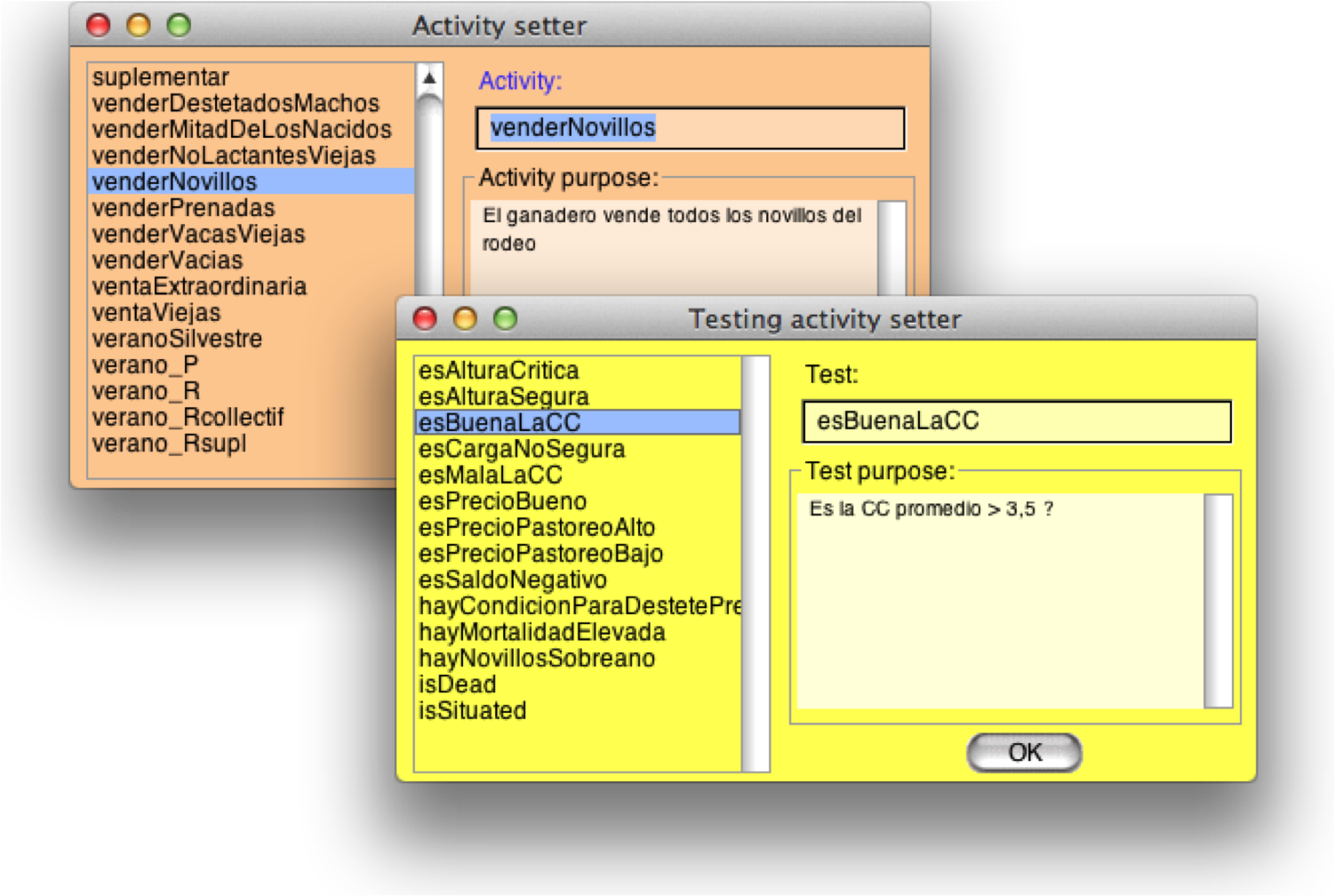
The activity setter displays a list of methods
belonging to the target class (i.e. Producer). This list
is set up automatically by Cormas that inspects all the
simple methods (without argument) defined within the
class and its super-classes. By clicking on a name, the
purpose of the associated method is displayed. It is
also possible inspect the method’s code by right
clicking on it. The design is
incremental: saving a new diagram generates a new method
of the agent that is immediately available and can be
called in turn (i.e. future activity setter will display
this new method name). A right-click on an activity or a
decision point opens either a code editor targeting the
selected operation, or another diagram editor displaying
the previously saved activities.
Therefore, the user can draw a transition from the
given node to another. When starting from a decision
point, he will create two transitions: one for which the
answer of the test is true (green) and one for
false (red). When saving the new diagram,
Cormas checks if the graph is coherent, then it
generates two operations in the target class: one to
store the diagram and one to execute it. Thus, from
basic operations already defined by the modeler, anyone
may generate new upper level behavior without any
programming skills.
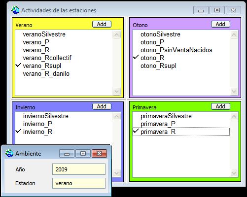
To edit the diagrams or choose which activities will be
used during the simulation, the user selects the names
of the methods that will be implemented at each station:
|